Comparing to NONMEM (bioav & lags)

[dvaish]

Hello there! I am new to Pumas and have trying to validate some of my previous results from NONMEM with Pumas. I have read through the docs nearly 10 times, and I got some of my other models to work, but for some reason, one of my drugs is producing results that are consistently too low. I cannot seem to identify the structural difference between the models that could be causing this, and I have tested and ensured that the error model is not the cause.

Here is the NONMEM model:

$PROBLEM Simulation Levofloxacin PK 
$INPUT   ID TIME EVID AMT DV TAD DROP SEX AGE WT HT WAZW WHZ HAZW BAZW COUNTRY ; Dropped TAD HIV ... Country    
$DATA    ../pop_sample1000_test.csv IGNORE=@
; AMT in mg
; DV in ug/mL or mg/L
; TIME in hours

$SUBROUTINE ADVAN6 TOL=5

$MODEL      NCOMP=4
            COMP=(DEPOT DEFDOS) 
            COMP=(CENTRAL DEFOBS)
            COMP=(PERIPH) 
            COMP=(AUC)

$PK
BSIZE1 = WT/12 ; This needed to be changed to 12 kg based on the study. see footnote a in table 2. 
EXPO   = 0.75

CLHIV  = 1 + 0*THETA(8)

; AGE EFFECT 
GAM     = THETA(11)
PMAGE50 = THETA(10)
MAT     = AGE**GAM/(PMAGE50**GAM + AGE**GAM) ; AGE in months 

; START PK
TVCL = THETA(1)*CLHIV*MAT*BSIZE1**EXPO ; added maturation on CL, removed HAZ.
CL   = TVCL*EXP(ETA(1))           ; CL, L/h [systemic clearance]

TVV  = THETA(2)
V    = TVV*BSIZE1*EXP(ETA(2))           ; V, L [central volume]

TVKA = THETA(3)           ; KA, 1/h [absorption rate]
KA   = TVKA*EXP(ETA(3))
 
TVVP = THETA(6)
VP   = TVVP*BSIZE1*EXP(ETA(4))

TVQ  = THETA(7)
Q    = TVQ*BSIZE1**EXPO*EXP(ETA(5))

TVF1 = 1
F1   = TVF1*EXP(ETA(6))

K20  = CL/V
K23  = Q/V
K32  = Q/VP

ALAG1 = THETA(9)*EXP(ETA(7))

$DES

DADT(1) = -KA*A(1)
DADT(2) = KA*A(1)-K20*A(2)-K23*A(2)+K32*A(3) 
DADT(3) = K23*A(2)-K32*A(3)
DADT(4) = A(2)/V

$ERROR 

REP = IREP
AUC = A(4)

; Proportional Residual Error model
CP    = A(2)/V
IPRED = CP 
PROP  = THETA(4)
ADD   = THETA(5)

W     = SQRT(PROP**2*IPRED**2+ADD**2)
IRES  = DV - IPRED
IWRES = IRES/W
Y     = IPRED + W*EPS(1)

$THETA  ; you need to change CL, V, Prop, Add, VP, Q ...
 4.7    ; 1 CL,L/h [systemic clearance]
 19.2   ; 2 Vc,L [central volume]
 1.61   ; 3 Ka
 0.116  ; 4 PROP 
 0.0160 ; 5 ADD 
 2.40   ; 6 VP
 0.796  ; 7 Q
 -0.159 ; 8 HIV on CL, study found 15.9% decrease in CL
 0.242  ; 9 ALAG
 10.6   ; 10 PMAGE50
 3.39   ; 11 GAMMA

$OMEGA  
 0.023  ; CL IIV these need to be converted. 15% CV = .15^2 = 
 0 FIX  ; V IIV 
 0.420  ; KA IOV ... we might want to consider inputting the BOV but for now it is fine.
 0 FIX  ; VP
 0 FIX  ; Q
 0.048  ; F1
 1.69   ; ALAG IOV

$SIGMA  1  FIX ; RV (use 20% CV as init est)
$SIM ONLYSIM NSUB=100 (12345)
$TABLE NOPRINT ONEHEADER FILE=simtab ID TIME EVID AMT TAD DV IPRED CP WT AUC REP WT AGE 

And here is the Pumas model;

model = @model begin
    @param begin
        tvcl    ∈ RealDomain(lower = 0) ; 1
        tvv     ∈ RealDomain(lower = 0) ; 2
        tvka    ∈ RealDomain(lower = 0) ; 3
        σ_prop  ∈ RealDomain(lower = 0) ; 4
        σ_add   ∈ RealDomain(lower = 0) ; 5
        tvvp    ∈ RealDomain(lower = 0) ; 6
        tvq     ∈ RealDomain(lower = 0) ; 7
        clhiv   ∈ RealDomain(lower = 0) ; 8
        alag    ∈ RealDomain(lower = 0) ; 9
        pmage50 ∈ RealDomain(lower = 0) ; 10
        γ       ∈ RealDomain(lower = 0) ; 11
        Ω      ∈ PDiagDomain(7)
    end

    @random begin
        η ~ MvNormal(Ω)
    end

    @covariates WT AGE

    @pre begin
        BSIZE1 = WT / 12
        EXPO = 0.75
        
        CLHIV = 1 + 0 * clhiv
        
        VP    = tvvp * BSIZE1                         * exp(η[4])
        Q     = tvq * (BSIZE1^0.75)                   * exp(η[5])
        MAT   = (AGE^γ) / ((pmage50^γ) + (AGE^γ))
        
        CL    = tvcl * CLHIV * MAT * (BSIZE1^0.75)    * exp(η[1])
        V     = tvv * BSIZE1                          * exp(η[2])
        KA    = tvka                                  * exp(η[3])
        
        K20   = CL / V
        K23   = Q / V
        K32   = Q / VP

        tvf1  = 1
        
        bioav = (Depot = tvf1 * exp(η[6]),)
        lags  = (Depot = alag * exp(η[7]),)
    end
    
    @dynamics begin
        Depot'       = -KA*Depot
        Central'     =  KA*Depot - Central*K20 - Central*K23 + K23*Peripheral
        Peripheral'  =  K23*Central - K32*Peripheral
        AUC'         =  Central / V
    end

    @vars begin
        conc  = Central / V
        auc   = AUC
    end

    @derived begin
        cp = @. Central / V
        dv ~ @. Normal(cp, sqrt(σ_add^2 + (cp*σ_prop)^2))
    end
end

fixeffs = (
    tvcl    = 4.7,
    tvv     = 19.2,
    tvka    = 1.61,
    σ_prop  = 0.116,
    σ_add   = 0.0160,
    tvvp    = 2.4,
    tvq     = 0.796,
    clhiv   = -0.159,
    alag    = 0.242,
    pmage50 = 10.6,
    γ       = 3.39,
    Ω       = Diagonal([0.023, 0, 0.420, 0, 0, 0.048, 1.69]),
)

obs = simobs(model, population, fixeffs, obstimes = 0:4:24) |> DataFrame

I apologize in advance if this post is too lengthy or otherwise out of the scope of what everyone can help with, but I appreciate any advice in advance, thank you!

Here is a histogram comparing the distributions of AUC between a single run of Pumas and a single run of NONMEM

And here is a histogram comparing the median AUC of a single Pumas run to the distribution of median AUC of 100 simulation runs in NONMEM

Thank you again!

[vijay]

hi Dhruv,

Welcome to the community and thank you for the detailed message.

Could you please clarify the time vector of the simulation you set up for your NONMEM dataset.

Best,
Vijay

[dvaish]

Hi Vijay! Thank you for the prompt response.

The NONMEM dataset has dose times [0, 24] and obs times [0, 4, 8, 12, 16, 20, 24]

Here is the population constructor I used in Julia for Pumas (reads from a DataFrame of individuals containing demographic data in corresponding columns)

function dose(WT, AGE)
    function amt(WT, AGE)
        return WT * 20
    end
    return DosageRegimen(amt(WT, AGE); time = 0:24:24)
end

function population_constructor(subjects)
    population = Subject[]
    for row in eachrow(subjects)
        subject = Subject(;
            id = row.ID, 
            events = dose(row.WT, row.AGE), 
            covariates = (WT = row.WT, AGE = row.AGE)
        )
        push!(population, subject)
    end
    return population
end

population = population_constructor(subjects[1:1000, :])

[benjaminrich]

The first thing I would do is simulate a single subject with each model, setting all random effects to 0, and see if the simulated concentrations match up. Have you tried that? On inspection, the models do look the same to me (I don’t see any obvious errors).

[dvaish]

Hi Benjamin!

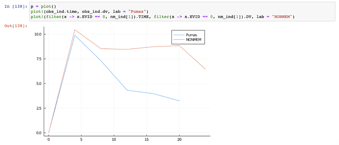
This was very insightful advice. I completed the steps to set random effects to zero (set the Omega vector to all zeros in Pumas and fixed the Omega block to all zeros in NONMEM). The results seem to show that the concentration in Pumas decays much faster after the dose event as compared to NONMEM. This seems to be causing the Pumas AUC to be significantly lower than the AUC in NONMEM as referenced in my first post. However, I cannot seem to identify the component of my model in Pumas / NONMEM that could be causing this difference.

Here is the plot for comparison:

Here is the difference in AUC:

And here is the difference in DV for reference:

I guess my question is: Is this due to some misspecification in my model or simply due to NONMEM and Pumas converging to different solutions?

[benjaminrich]

I think I’ve spotted the error. It’s in the Pumas model, in this line:

        Central'     =  KA*Depot - Central*K20 - Central*K23 + K23*Peripheral

The last term has K23 where it should be K32. In other words, it should read:

        Central'     =  KA*Depot - Central*K20 - Central*K23 + K32*Peripheral

[pkofod]

That does seem right @benjaminrich ! Good catch.

Let me add another way to check or verify this. You could use the Depots1Central1Periph1 analytical solution and add on the AUC calculations as a numerical calculation

@dynamics Depots1Central1Periph1 begin
    AUC' = Central/V
end

[dvaish]

Hi All!

Thank you very much for the advice. In fact, @benjaminrich that was the issue. I am now getting values much more closely in the range of what I would expect! Thank you also to @pkofod! I tried running the model with this preset, but after consulting the documentation, I determined that the built in specification for that model is different from how I have defined it in NONMEM (uses (CL + Q)/Vc for K20 whereas I am using CL/Vc

Here are the final results:
TIME vs. CP

AUC Distribution

Median AUC’s

These Pumas results appear slightly lower on average than the NONMEM results, but within the margin of error. Thank you all for all your help!

[benjaminrich]

Hi @dvaish. This is not resolved in my opinion. The CP curves should completely overlap (the “margin of error” should be much smaller than what you are seeing). So I would continue to look for an explanation for the difference you are observing.

[benjaminrich]

For the TIME vs. CP figure you generated, what AGE and WT did you use?

[dvaish]

Hi @benjaminrich
WT = 8, AGE = 5

[dvaish]

Actually you are absolutely correct @benjaminrich, it appears that in rerunning the model I misspecified one of the parameters, and in fact, upon rerunning it just now, I have achieved exactly the correct answer.

The lines are completely indistinguishable! Thank you so much, this was incredibly helpful I look forward to using this tool much more in the future!

[dvaish]

As a followup @benjaminrich or @pkofod, part of my modeling workflow is to use the NSUB=100 feature in NONMEM simulation, which allows for 100 separate simulations of the data (where I got the AUC distributions). Can this be replicated by some option in Pumas or should I just be bootstrapping and rerunning the simulation 100 times ?

[benjaminrich]

That is excellent, just what I was hoping and expecting.

For the simulation replicates, you can try something like this:

nsub = 100
sim_replicates = [DataFrame(simobs(model, population, fixeffs, obstimes = 0:4:24)) for i in 1:nsub]
sim_replicates = vcat(sim_replicates...)